


The agile radar and its timeless fundamentals – the radar range equation.
By Giovanni D’Amore, Market Development Manager, Keysight
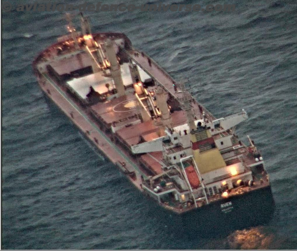
Radar has come a long way from the late 19th century and has evolved into a host of technologies supporting a broad range of applications today. Applications range from the simple, inexpensive and small size continuous-wave (CW) radar used by law enforcers to ensnare speed offenders, to the complex active phased arrays used in ground based, naval and airborne radar systems. A typical active phased array or active electronically steered array (AESA) consists of hundreds or thousands of transmit/receive (T/R) modules, made possible with high performance solid-state devices.
As radar technologies move up to higher frequencies and wider bandwidths, new applications previously unimaginable have emerged. The low-cost and non-ionizing ultra-wide band microwave imaging provides different insights as compared to existing imaging techniques and offers promising applications in the field of medical and healthcare. The radar gesture recognition with resolution down to the sub-millimeter range offers consumers new ways of interfacing with devices1. Radar technologies also enable autonomous driving and drones with anti-collision and ranging capabilities. The THz band with its unique spectral properties towards chemical and biological contents excites both scientific and non-scientific communities alike with potential applications in imaging, sensing and detection. As radar gain new applications, we will provide a brief review on the timeless fundamentals of radar.
Principle of operation
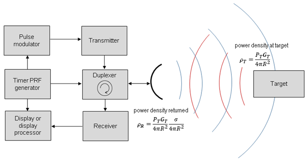
The essence of radar is the ability to gather physical information about a target or multiple targets — location, speed, direction, shape, identity or simply presence. This is achieved by processing reflected electromagnetic waves in the case of primary radars, or from a transmitted response in the case of secondary radars. In most implementations, a pulsed-RF or pulsed-microwave signal is generated by the radar system, beamed toward the target in question and collected by the same antenna that transmitted the signal.
The essential block diagram of a pulse radar system is depicted in Figure 1. In this diagram, the master timer or PRF generator is shown as the central block of the system. The PRF generator plays an important role to time synchronize all components of the radar system through connections to the pulse modulator, duplexer or transmit/receive switch, and the display processor. In addition, connections to the receiver would provide gating for front-end protection or timed gain control such as sensitivity time control (STC).
The radar range equation explained
The radar range equation describes the important performance variables of a radar and provides a basis for understanding the measurements that are made to ensure optimal performance. The equation can be presented in many different forms. Equation 1 shows one form of the radar range equation which gives the maximum radar range in meters. To better understand the given equation and the assumptions used, readers are encouraged to follow the derivation2.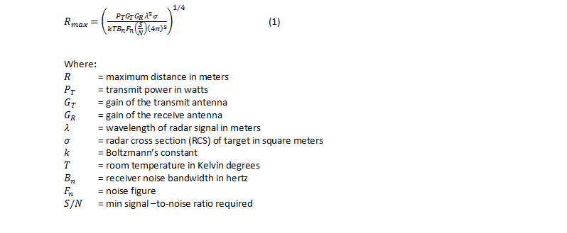
The derivation starts by analyzing a simple spherical scattering model of propagation for an isotropic radiator, or point-source antenna. Because radar systems use directive antennas to focus radiated energy onto a target, the gain of the antenna is defined as the ratio of power directed toward the target compared to the power from an ideal isotropic antenna. The equation accounts for the directive gain of the antenna with and for transmit and receive, respectively. If the same antenna is used for transmit and receive, both terms can be replaced with , for simplicity.
Some of the transmitted power density that strikes the target will be reflected off in various directions and some of the energy will be reradiated back to the radar system. The amount of this incident power density that is reradiated back to the radar is a function of the radar cross section (RCS or ) of the target. RCS ( ) has units of area and is a measure of target size, as seen by the radar.
A portion of this signal reflected by the target will be intercepted by the radar antenna. This signal power will be equal to the return power density at the antenna multiplied by the effective area of the antenna. The primary factor limiting the receiver is noise and the resulting signal-to-noise ( ) ratio.
The noise power (theoretical limit) at the input of the receiver is described as Johnson noise or thermal noise. It is a result of the random motion of electrons, and is proportional to temperature. The available noise power at the output of the receiver will always be higher than the thermal Johnson noise. This is due to the extra noise generated within the receiver. Hence, Equation 1 factored in noise generated within the receiver by multiplying the Johnson noise power by the noise factor and gain of the receiver.
Equation 1 describes the maximum target range of our radar based on transmitter power, antenna gain, RCS of the target, system noise figure, and minimum signal-to-noise ratio. In reality, this is a simplistic model of system performance. There are many factors that will also affect system performance including modifications to the assumptions made to derive this equation. Two additional items that should be considered are system losses and pulse integration that may be applied during signal processing. Losses in the system will be found both in the transmit path and in the receive path .
In a classical pulsed radar application, we could assume that multiple pulses would be received, from a given target, for each position of the radar antenna (because the radar’s antenna beamwidth is greater than zero, we can assume that the radar will dwell on each target for some period of time) and therefore could be integrated together to improve the performance of the radar system. As this integration may not be ideal, an integration efficiency term based on the number of pulses integrated will be used to describe integration improvement. Including these terms, the radar equation yields:
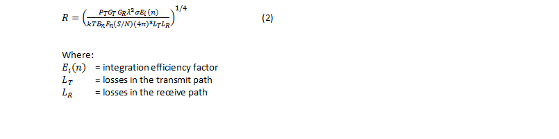
For multiple-antenna radars, the radar range would grow proportionally to the number of elements, assuming equal performance from each element.
Making sense of the radar range equation
The signal power at the radar receiver is directly proportional to the transmitted power, the antenna gain (or aperture size), and the radar cross section (RCS) (i.e., the degree to which a target reflects the radar signal). Perhaps more significantly, it is indirectly proportional to the fourth power of the distance to the target. Given the large attenuation that occurs while the signal is traveling to and from the target, having high power is very desirable. However, having high power is difficult due to practical problems such as heat, voltage breakdown, dynamic power requirements, system size and cost.
In the follow-up topic, we will cover the characteristics, compression techniques and measurement of the pulsed radar signal.
Reference: